In Machine Learning, why is Regularization called Regularization?
Introduction
Many newcomers to machine learning know about regularization, but they may not understand it yet. In particular, they may not know why regularization has that name. In this post we discuss the numerical and statistical significance of regularization methods in machine learning and more general statistical models. We’ll try to introduce why one may want to use regularization methods in the first place and how to interpret the fitted model from a statistical point of view.
The post will be long because there are a lot of cute nooks and crannies, and we’ll assume you know your linear algebra. However, if you already know what an inner product is then we think this post will be worth your time.
Matrices and Linear Ill-Posed Problems
Suppose that we have a matrix \(A\in \mathbb{R}^{N \times p}\), a vector \(y\in \mathbb{R}^N\), and that we seek a vector \(\beta\in\mathbb{R}^p\) such that \(A\beta = y\). How would one solve this problem? One answer might be to simply apply the inverse matrix to both sides of the equation: \(\beta = A^{-1}y\). However, there are three problems with this:
- A matrix inverse \(A^{-1}\) may not exist.
- Even if the matrix inverse exists it can be extremely expensive to calculate this inverse and apply the result to \(y\).
- Even if we are somehow able to calculate \(A^{-1}y\) the solution may not be very stable. Small numerical changes in either \(A\) or \(y\) may lead to large changes in the solution \(\beta\).
Issue 2 above is not really a problem in the sense that one should never really need to find \(A^{-1}\) to compute \(A^{-1}y\). Instead the most efficient numerical algorithms typically compute \(A^{-1}y\) by using special factorizations of \(A\), such as QR decomposition.
The other two issues are very important and are inextricably linked to each other and to regularization in machine learning.
Issue 3 means just what is says: that the solution \(\beta\) may change a lot if the known data \(A\) and/or \(y\) only change a little.
Issue 1 means that the matrix is not invertible. A matrix that is not invertible is called singular. A matrix that is invertible is usually called nonsingular, but a less common synonym is regular and this is where the name regularization comes from. When a matrix is singular it means that the problem \(A\beta = y\) may have either no solution at all or have at least 2 distinct solutions.
Any one of these issues being true means that the linear problem \(A\beta = y\) is ill-posed in the sense that it violates Hadamard’s conditions for a well-posed problem. To be well-posed:
- A problem must have a solution
- The solution must be unique
- The solution’s behavior must be stable/continuous with respect to the data
These conditions are of extreme practical importance. They basically define what it means for a problem to be solvable in practice. In the case of the linear algebra problem above regularization means “making the matrix regular” so that these conditions will hold true on the regularized problem. That’s where the name comes from.
Ok, cool but why are these conditions important to ML or statistics? Consider the case of Maximum Likelihood Estimation (MLE) of a parametric model (although the lesson applies more generally):
- In MLE we estimate a model’s unknown parameters by maximizing the log-likelihood. If no such maximizing values of the parameters can be found then the optimization problem does not have a solution and we can not obtain estimates for the unknown parameters to begin with! So, mirroring the first Hadamard condition, we require a maximizer to exist.
- Non-Bayesian statistical models naturally assume that a single fixed set of parameters exists that specifies the relevant distributions. If MLE gives multiple sets of parameters that maximize the likelihood (as happens in the presence of multiple local maxima) we may have no way to tell which maximizer is the one that estimates the actual parameters the best! So, mirroring the second Hadamard condition, we require the maximizer to be unique.
- Statistical models assume that data is in part random and so is subject to changes. If the estimated values of the parameters change a lot when the data changes a little then it’s impossible to tell when the MLE estimated parameters are in fact good estimates of the true parameters and when they are not! So, mirroring the third Hadamard condition, we require the maximizer to be stable with respect to changes in the data used for the fit.
Regularization is one way to change the problem so that these conditions are met.
Some examples
Ok, let’s look at some examples!
Shifting the eigenvalues of a Symmetric Matrix
Suppose we are asked to solve the linear inverse problem from above \(A\beta = y\), but that this time \(A\in \mathbb{R}^{N\times N}\) is a symmetric matrix. The spectral theorem for symmetric matrices tells us that \(A\) can be represented as
\[ A = QDQ^T \] where \(Q\) is an orthogonal matrix and \(D\) is a diagonal matrix. Moreover, the columns of \(Q\) are the eigenvectors of \(A\), and the diagonal elements of \(D\) are the corresponding (real) eigenvalues. Here’s a proof if you care for it.
This representation shows us exactly what the theoretical difficulty is in the inverse problem. Inverting \(Q\) is easy. Indeed orthogonal matrices are always invertible, with the inverse given by the transpose: \(Q^{-1} = Q^T\). The geometric significance of orthogonal matrices comes from the fact (basically their definition) that they preserve the inner product of vectors: If we denote the inner product by \(\langle \cdot,\cdot\rangle\) then for any \(x,y \in R^N\)
\[ \langle x, y \rangle = \langle Qx, Qy \rangle \] Thus (using the definition of the transpose) \(\langle x, y \rangle = \langle Q^TQx, y \rangle\). Since this holds for any \(y\), then \(x = Q^TQx\) for all \(x\). Since this holds for all \(x\) then \(Q^TQ = I\) and so \(Q^T\) is the inverse of \(Q\).
No, the difficulty is simply in inverting the diagonal matrix \(D = \text{diag}(\sigma_1, \sigma_2, ..., \sigma_N)\). If none of the eigenvalues \(\sigma_i\) are \(0\) then \(D^{-1} = \text{diag}(\sigma_1^{-1}, \sigma_2^{-1}, ..., \sigma_N^{-1})\). In this case there isn’t any direction that \(D\) (and hence \(A\)) squashes into \(0\). However, if some of the \(\sigma_i\)’s are \(0\) then we can not invert \(D\) and the problem will fail to satisfy at least one of the first 2 Hadamard conditions. Even if none of the \(\sigma_i\)’s are exactly \(0\), some may be numerically very close to \(0\) in comparison to the others. In that case the value of their reciprocals may be enormously large and may lead to numerical instability in the problem, violating the 3rd Hadamard condition. This would be a big problem in practice because computers hate mixing floating point numbers that are drastically different in size.
To address this issue we note that we can shift the eigenvalues of \(A\) by adding a multiple of an identity matrix:
\[ A \to A + \lambda I \] If \(\sigma\) is an eigenvalue of \(A\) then \(\sigma+\lambda\) is an eigenvalue of \(A+\lambda I\). This is because every vector is an eigenvector of \(I\): If \(Av = \sigma v\) then trivially \(\lambda Iv = \lambda v\), so adding gives \((A+\lambda I)v = (\sigma + \lambda)v\). This can also be seen form the representation above: \[ A + \lambda I = QDQ^T + \lambda QQ^T = Q(D + \lambda I)Q^T = Q\tilde{D}Q^T \] where \(\tilde{D}= \text{diag}(\sigma_1 + \lambda, \sigma_2 + \lambda, ..., \sigma_N + \lambda)\). Therefore, if we choose \(\lambda > \min\{\sigma_1, \sigma_2, ..., \sigma_N\}+ \delta\) for some \(\delta > 0\), then all the shifted eigenvalues satisfy \(\sigma_i + \lambda > \delta > 0\) and the new shifted problem
\[ (A+\lambda I)x = y \] will be solvable with solution given by \[ x = Q(D + \lambda I)^{-1}Q^Ty \] If \(\lambda\) is sufficiently large this inverse will exist and will be numerically stable (all of the eigenvalues will have been shifted away from 0).
Making the change \(A \to A + \lambda I\) regularized the problem into one that satisfied Hadamard’s conditions, which is fundamentally the point of regularization. The change we made was essentially to replace the \(A^{-1}\) with the approximation \((A+\lambda I)^{-1}\), but we could have used other approximations as well, for example partial sums of the Neumann Series Expansion of the \(A^{-1}\). Regardless, the general principle illustrated above is basically to replace one problem by an approximate problem that does not suffer the same existence/stability issues.
Regularization as a perturbation of an invertible matrix
Above we regularized the ill-posed problem \(A\beta = y\) by replacing it with the problem \((A+\lambda I)x = y\). Let’s go a bit deeper with this process.You may skip this section on your first read.
Dividing by \(\lambda\), the problem \((A+\lambda I)x = y\) is equivalent to the problem
\[ (\epsilon A+I)x = \epsilon y \] where \(\epsilon := \frac{1}{\lambda}\). When \(\lambda\) is large \(\epsilon\) is small, and vice versa. Hence for large \(\lambda\) the matrix \(\epsilon A+I\) can be seen as a small perturbation from the identity matrix \(I\).
Now because \(I\) is invertible then for a small enough \(\epsilon\) (and hence for a large enough \(\lambda\)) the preturbed matrix \(\epsilon A+I\) is also invertible! Why? That’s a great question! The previous section gave one proof, but there are some much nicer ways to see why:
Proof: Consider the function \[ \det:\mathbb{R}^{N\times N} \to \mathbb{R} \] that maps a matrix to it’s determinant. Because the space \(\mathbb{R}^{N\times N}\) of \(N\times N\) matrices is just the Euclidean inner product space \(\mathbb{R}^{N^2}\) with some extra algebraic structure, and because \(\det(A)\) is a polynomial function of the elements of a matrix \(A\), \(\det\) is a continuous function on \(\mathbb{R}^{N\times N}\).
By Cramer’s Rule, a matrix \(A\) is invertible if and only if \(\det(A) \ne 0\). Because \(\det\) is a continuous function on \(\mathbb{R}^{N\times N}\) then the set of invertible matrices is an open subset of \(\mathbb{R}^{N\times N}\)! Hence for every invertible matrix \(L\in\mathbb{R}^{N\times N}\) and every arbitrary matrix \(A\in\mathbb{R}^{N\times N}\) there exists an \(\epsilon_0 > 0\) such that for all \(\epsilon < \epsilon_0\) the matrix \(\epsilon A+L\) is invertible. QED
There’s a version of the theorem in Banach spaces, but we don’t need it.
Noticed that the only thing we needed about the matrix \(I\) in the above proof was that it was invertible. Therefore, we never needed to restrict attention to just the identity matrix \(I\), but could have used any invertible matrix to regularize the problem:
\[ (A+\lambda L)x = y \]
where \(L\) is any convenient invertible matrix. Below, where we regularize OLS, we are not restricted to using the identity matrix \(I\) to regularize, but can use any invertible symmetric matrix (preferably one that is positive definite so that a minimizer continues to exist).
\(L^2\)-regularization of OLS
With this example we begin moving towards the statistical part of the post. One of the most widely known examples of regularization is what is often called \(L^2\)-regularization, or Tikhonov regularization of Ordinary Least Squares.
Suppose \(Y\) is a real valued random variable and \(\vec{X}\) is a random vector with values in \(\mathbb{R}^p\). Suppose that we have the conditional relationship
\[ Y \ \ | \ \ \vec{X} \sim \mathcal{N}(\ \langle \vec{X} , \beta\rangle \ ,\ \sigma^2) \]
where \(\mathcal{N}(\mu, \sigma^2)\) denotes the univariate normal distribution with mean \(\mu\) and variance \(\sigma^2\). Here (and everywhere else) the symbol \(\langle v,w\rangle\) represents the inner product of two vectors \(v\) and \(w\). This is the most natural probability model that leads to linear regression. In practice the parameters \(\beta\) and \(\sigma\) that specify this conditional distribution are unknown and it is desired that they be estimated from data.
In this canonical situation we assume that we have a data set \(\{ (Y_i, \vec{X}_i)\}_{i = 1}^N\) consisting of samples generated independently of one another from a fixed multivariate distribution for \((Y, \vec{X})\) (i.e. we assume our data was sampled IID). To fit the unknown parameters we use MLE. We may choose to use the conditional density \(p(Y|\vec{X})\) in the likelihood and this would make it conditional MLE. Or we may choose the unconditional multivariate density \(p(Y, \vec{X})\). However, if we assume that the marginal distribution of \(\vec{X}\), (i.e. \(p(\vec{X})\)), does not depend on either \(\beta\) or \(\sigma\) then because \(p(Y,\vec{X}) = p(Y|\vec{X})p(\vec{X})\) building the likelihood using either \(p(Y|\vec{X})\) or \(p(Y,\vec{X})\) will lead to the same maximization problem because they differ by a constant factor (constant in \(\beta\) and \(\sigma\) that is). So we will use the conditional density \(p(Y|\vec{X})\).
Because the data is assumed to be generated IID then the full likelihood of the data is
\[ \mathcal{L}(\beta, \sigma\ |\ \{ (Y_i, \vec{X}_i)\}) = \prod_{i = 1}^N p(Y_i|\vec{X}_i) = \prod_{i=1}^N\frac{1}{\sigma\sqrt{2\pi}}e^{-\frac{1}{2}\big(\frac{Y_i - \langle \vec{X}_i , \beta\rangle}{\sigma}\big)^2} = \frac{1}{(\sigma^22\pi)^{N/2}}e^{\sum_{i=1}^N-\frac{1}{2}\big(\frac{Y_i - \langle \vec{X}_i , \beta\rangle}{\sigma}\big)^2} \] Because the function \(f(x) := -\log(x)\) is decreasing we may instead minimize the negative of the log of this expression: \[ -\log(\mathcal{L}(\beta,\sigma\ |\ \{ (Y_i, \vec{X}_i)\})) = \frac{N}{2}\log(\sigma^22\pi) + \frac{1}{2\sigma^2}\sum_{i=1}^N\bigg(Y_i - \langle \vec{X}_i , \beta\rangle\bigg)^2 \] We first minimize with respect to \(\beta\) as this is necessary to do first before finding the minimizing value of \(\sigma\). To do this we need to minimize the only term that depends on \(\beta\), namely the sum of squares \(SSE(\beta) := \sum_{i=1}^N\bigg(Y_i - \langle \vec{X}_i , \beta\rangle\bigg)^2\) (hence Least Squares regression).
A geometric interlude
Before we do that, let’s think about what the expression \(SSE(\beta)\) is. The term \(\langle \vec{X}_i , \beta\rangle\) is linear in the unknowns \(\beta\), and hence so is \(Y_i - \langle \vec{X}_i , \beta\rangle\). Therefore, the square \(\bigg(Y_i - \langle \vec{X}_i , \beta\rangle\bigg)^2\) is quadratic in \(\beta\). Thus since the full expression \(\sum_{i=1}^N\bigg(Y_i - \langle \vec{X}_i , \beta\rangle\bigg)^2\) is a sum of quadratic functions in \(\beta\) it too is a quadratic function in \(\beta\). Since all terms in the sum are squares, the full sum is never negative and its graph in \(\beta\) is a non-hyperbolic paraboloid. Usually such shapes look like bowls. However, some can degenerate so that they become flat in one or more directions. Here’re some examples in R:
Non-degenarte paraboloids look like this:
nice.paraboloid = function(x,y)
{
    return(x^2+0.5*y^2)
}
x = y = seq(from = -4, to = 4, by = 0.2)
z = outer(x, y, nice.paraboloid)

persp(x, y, z,
      main="Plot of a Non-degenerate 2D Paraboloid",
      theta = 30, phi = 15,
      col = "springgreen", shade = 0.5)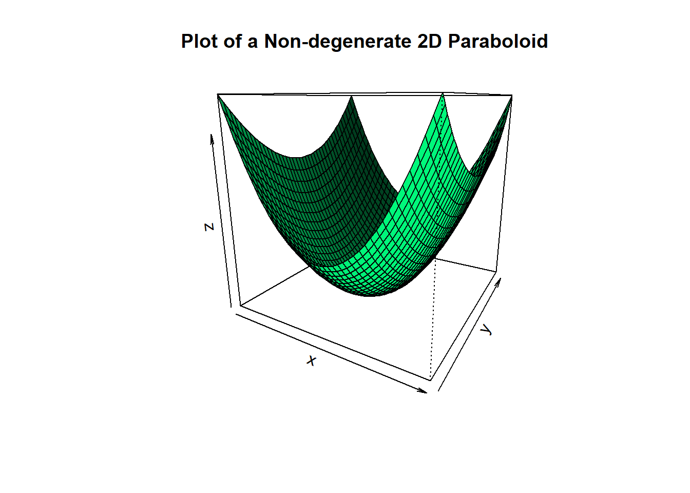
We can see such a paraboloid is bowl shaped. More technically it’s strictly convex, with a clear unique minimum point. However, paraboloids can degenerate so that they flatten out in some directions:
degenerate.paraboloid = function(x,y)
{
    return(x^2) #Does not change value as y changes
}
x = y = seq(from = -4, to = 4, by = 0.2)
z = outer(x, y, degenerate.paraboloid)

persp(x, y, z,
      main="Plot of a Degenerate 2D Paraboloid",
      theta = 30, phi = 15,
      col = "springgreen", shade = 0.5)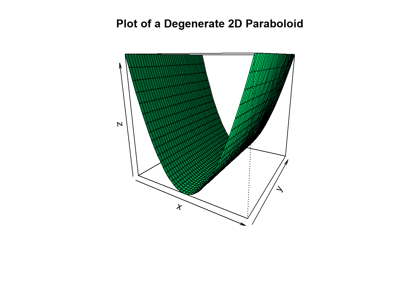
In this example we changed the coefficient of \(y\) from 0.5 to 0. The result is that in the \(y\)-direction the paraboloid flattened out and it no longer looks bowl shaped. Instead there are infinitely many minimum points all on the axis \(\{(x,y): x = 0\}\). Note that if instead of making the coefficient of \(y\) equal to 0 we had made it a positive number very close to zero then the mimima would become unique but would become hard to distinguish from nearby points:
tricky.paraboloid = function(x,y)
{
    return(x^2+ 0.05*y^2) #Notice the coefficient of y is quite small
}
x = y = seq(from = -4, to = 4, by = 0.2)
z = outer(x, y, tricky.paraboloid)

persp(x, y, z,
      main="Plot of a Nearly-Degenerate 2D Paraboloid",
      theta = 30, phi = 15,
      col = "springgreen", shade = 0.5)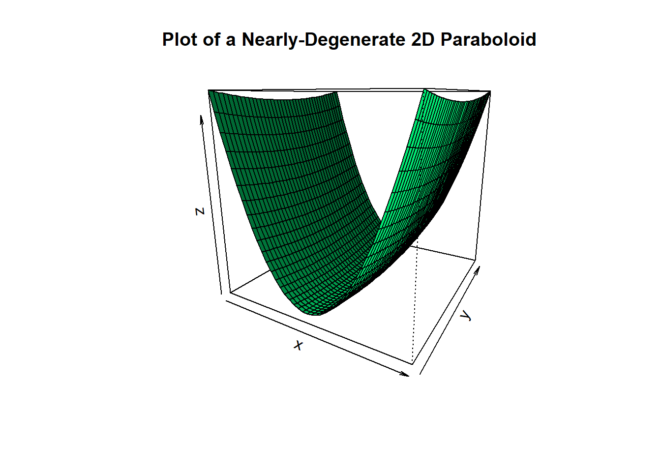
These pictures show what can go wrong with the minima of quadratic functions like \(SSE(\beta)\) and why regularization may be needed. Now to get back to the minimizing the sum of squares \(SSE(\beta) = \sum_{i=1}^N\bigg(Y_i - \langle \vec{X}_i , \beta\rangle\bigg)^2\). If you’re reading this article I’m going to assume you’ve seen this derivation before so I’ll move a bit fast.
First we define \(Y\in \mathbb{R}^{N\times 1}\) with \(i\)-th component equal to \(Y_i\). (Note an abuse of notation we are making: earlier \(Y\) denoted a real valued random variable, but now we are using the same symbol to denote the vector of the \(N\) realizations of this random variable.) In addition, let \(X\in \mathbb{R}^{N\times p}\) with \(i\)-th row equal to \(\vec{X}_i\). Then in matrix notation
\[ \sum_{i=1}^N\bigg(Y_i - \langle \vec{X}_i , \beta\rangle\bigg)^2 = (Y - X\beta)^T(Y - X\beta) \] Let \(\hat{\beta} = \text{argmax}_{\beta} \ \ (Y - X\beta)^T(Y - X\beta)\) be the sought after minimizer. Since \(\hat{\beta}\) is a minizer in the interior of the domain of \(SSE(\beta)\), the gradient of \(SSE(\beta)\) at \(\hat{\beta}\) must be 0:
\[ -2X^TY + 2X^TX\hat{\beta} = 0 \] therefore we obtain the normal equations
\[ X^TX\hat{\beta} = X^TY \]
This is basically the same linear algebra problem as before: If the inverse \((X^TX)^{-1}\) existed and was numerically nice then we can solve for \(\hat{\beta} = (X^TX)^{-1}X^TY\). However, if this matrix inverse does not exist (as can happen when we do not have enough rows/samples for the given number of columns/unknowns) then this formula is not useful.
But as before we can simply regularize by replacing the matrix \(X^TX\) by \(X^TX + \lambda I\) for some sufficiently large \(\lambda\). Actually since \(X^TX\) is non-negative definite1 and symmetric all of it’s eigenvalues are non-negative. So any \(\lambda > 0\) would be sufficient to shift the eigenvalues into positive numbers. Now the regularized problem becomes \((X^TX + \lambda I)\hat{\beta} = X^TY\). Therefore we get the regularized MLE solution:
\[ \hat{\beta}_{reg} := (X^TX + \lambda I)^{-1}X^TY \]
Does this regularized problem correspond to its own minimization problem? Yes! Working backwards, this new problem is equivalent to
\[ -2X^TY + 2X^TX\hat{\beta} + 2\lambda\hat{\beta}= 0 \] The left had side is the gradient of \((Y - X\beta)^T(Y - X\beta) + \lambda\sum_{j=1}^p\beta_j^2 = (Y - X\beta)^T(Y - X\beta) + \lambda \langle \beta, \beta\rangle\) at \(\beta = \hat{\beta}\) as can be checked. So the regularized problem corresponds to trying to minimize the expression \((Y - X\beta)^T(Y - X\beta) + \lambda\sum_{j=1}^p\beta_j^2 = (Y - X\beta)^T(Y - X\beta) + \lambda \langle \beta, \beta\rangle\). This of course is \(L^2\)-regularization. Thus we have derived \(L^2\)-regularization for OLS simply by seeking to transform the inverse problem that arises in OLS so that it may satisfy the Hadamard conditions.
An Illustrative Example
Below we can see geometrically what regularization does. The sum of squares expression \((Y - X\beta)^T(Y - X\beta)\) is quadratic in \(\beta\), but may have a graph that is a degenerate paraboloid. This is what causes it to have multiple minimizers in OLS and what makes the matrix \(X^TX\) singular (more on this point in the next section). However the expression \(\lambda\langle \beta, \beta\rangle = \lambda\sum_{j = 1}^p\beta_j^2\) is a strictly positive-definite quadratic form. Its graph is a non-degenerate bowl shaped paraboloid.
Adding a non-degenerate paraboloid to something that is not bowl shaped makes the second graph more bowl shaped! Moreover it shifts the minimum of the 2nd graph towards the mimimum of the bowl. As an illustration, let’s take a look at an example where this is easy to see.
rm(list = ls())
bumpy.function = function(x,y)
{
    return(sin(x)+sin(y))
}

nice.paraboloid = function(x,y)
{
    return(0.15*(x^2 + y^2)) #lambda = 0.15 is used
}

x = y = seq(from = -4, to = 4, by = 0.2)
bumpy = outer(x, y, bumpy.function)
paraboloid = outer(x, y, nice.paraboloid)
bumpy.plus.paraboloid = bumpy + paraboloid

persp(x, y, bumpy,
      main="Graph of a bumpy function with multiple minima",
      theta = 30, phi = 15,
      col = "springgreen", shade = 0.5)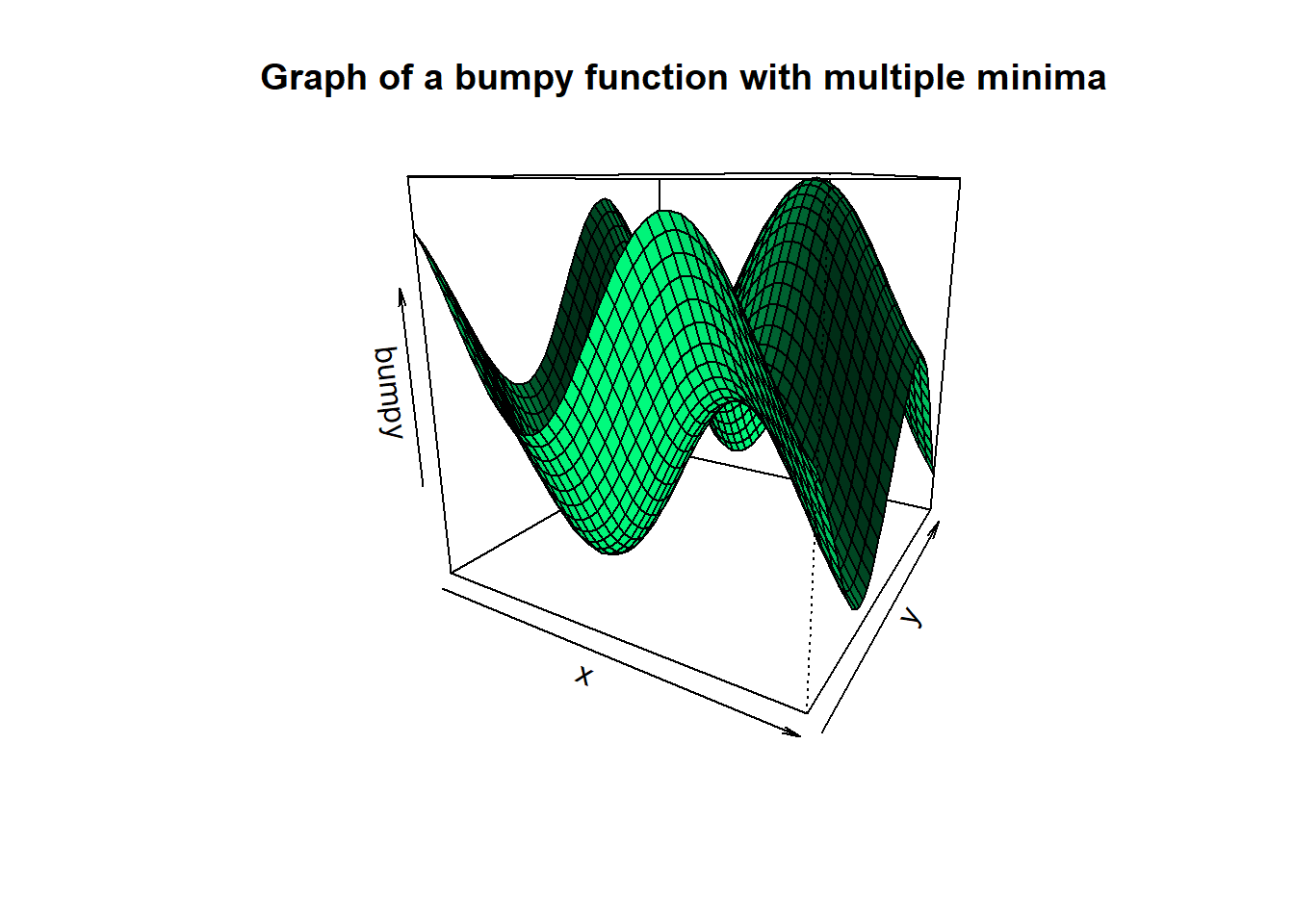
persp(x, y, paraboloid,
      main="Graph of a nice paraboloid",
      theta = 30, phi = 15,
      col = "springgreen", shade = 0.5)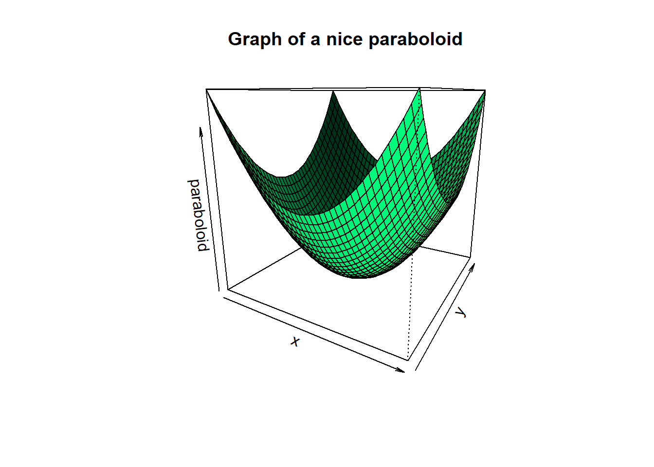
persp(x, y, bumpy.plus.paraboloid,
      main="Graph of a regularized bumpy function = bumpy function + paraboloid",
      theta = 30, phi = 15,
      col = "springgreen", shade = 0.5)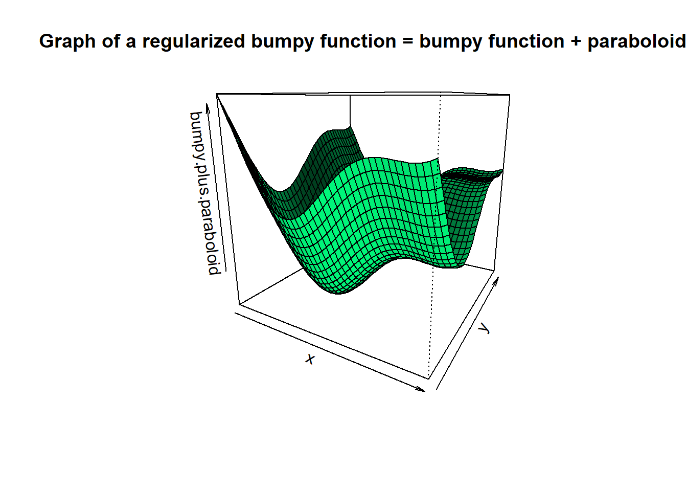
Here we see that the most important geometric aspect of the regularizing term \(\lambda\langle\beta, \beta\rangle\) is the fact that it is strictly convex!! Although we will not dwell on it, it is impossible to overstate the theoretical importance of the previous sentence. As a matter of fact, geometrically speaking it’s clear that had we added any strictly convex function to the bumpy function we would have gotten something more bowl shaped. We will not go further into it here but you should know that convexity is one of those properties in mathematics out of which entire fields are created.
The Hessian matrix and more complex models
In the OLS problem above the Maximum Likelihood estimator turned out to be the one that minimized the sum of squares expression \(SSE(\beta) := (Y - X\beta)^T(Y - X\beta)\). This expression can be expanded in matrix notation as
\[ Y^TY - Y^TX\beta - \beta^TX^TY + \beta^TX^TX\beta \]
We see that there is a quadratic term (\(\beta^TX^TX\beta\)) and the rest are terms with powers of \(\beta\) less than 2. The matrix of second derivatives of this expression (known as the Hessian matrix) is therefore just the matrix of coefficients of this quadratic term: \(X^TX\). This Hessian is exactly what was the star of the show in the OLS problem!
The Hessian of a function at a point tells us the convexity of the function at the point. If the Hessian is positive definite, then near the minimizing point the function is bowl shaped. If the Hessian is negative definite then near a maximizing point the function is shaped like an upside down bowl.
Moreover, The Hessian is always a symmetric matrix by the equality of cross-derivatives. So the previous point is really a statement about Hessian’s eigenvalues. In short, if the Hessian has all positive eigenvalues then it is positive definite and the function is bowl shaped near its minimizer.
The OLS Hessian matrix \(X^TX\) is symmetric and non-negative definite, so the graph of the sum of squares \(SSE(\beta) := (Y - X\beta)^T(Y - X\beta)\) can only fail to be bowl shaped near the minimizer \(\hat{\beta}\) if the matrix \(X^TX\) has eigenvalues that are equal 0 (or positive but close to 0 in the case numerical instability). In which case, the graph of \(SSE(\beta)\) is a degenerate non-hyperbolic paraboloid and there are multiple minimizing solutions \(\beta\).
Thus regularizing the matrix \(X^TX\) is just regularizing the Hessian matrix of the function \(SSE(\beta)\) we want to minimize!! This fact is what allows us to take the idea beyond OLS.
Indeed if \(f(\beta)\) is any 2nd order differentiable cost function in any machine learning model then by the linearity of the derivative
\[ \text{Hessian}(f + \lambda \langle \beta, \beta\rangle) = \text{Hessian}(f) + \lambda\text{Hessian}(\langle \beta, \beta\rangle) = \text{Hessian}(f) + \lambda I \]
There we used the fact that \(\text{Hessian}(\langle \beta, \beta\rangle) = \text{Hessian}(\sum_i^p \beta_i^2) = I\). Because \(f\) is almost arbitrary we see that we can apply \(L^2\)-regularization to a very large family of problems, with the goal being to regularize the Hessian of \(f\). As an example let’s look at some other kinds of regression problems. For OLS we assumed the conditional distribution \(Y \ \ | \ \ \vec{X} \sim \mathcal{N}(\ \langle \vec{X} , \beta\rangle \ ,\ \sigma^2)\), but we may have chosen a different conditional distribution.
If \(Y\) takes on only values in the set \(\{0,1\}\) then it is a Bernoulli random variable. This is the case in logistic regression where the conditional distribution of \(Y\) given \(\vec{X}\) is \[ Y \ \ | \ \ \vec{X} \sim \mathcal{B}(\ p = \phi(\langle \vec{X} , \beta\rangle) \ ) \]
where \(\mathcal{B(p)}\) is a Bernoulli distribution with probability of a positive event equal to \(p\), \(p = \text{E}[Y|\vec{X}] = \phi(\langle \vec{X} , \beta\rangle)\) is the probability of a positive event given \(\vec{X}\), and \(\phi(t) = \frac{e^t}{1+e^t}\) is the standard logit. In this case the conditional density \(p(Y|\vec{X})\) can be written as
\[ p(Y|\vec{X}) = p^Y\big(1 - p)\big)^{1-Y} =\phi(\langle \vec{X} , \beta\rangle)^Y\big(1 - \phi(\langle \vec{X} , \beta\rangle)\big)^{1-Y} \] So the negative log-likelihood is given by
\[ -\mathcal{l}(\beta) = -\sum_{i=1}^N Y_i\log(\phi(\langle \vec{X}_i , \beta\rangle)) + (1-Y_i)\log(1-\phi(\langle \vec{X}_i , \beta\rangle)) \]
This function may or may not look bowl shaped (i.e. strictly convex) near the \(\hat{\beta}\) that minimizes it. In case it doesn’t we can make it so by adding \(\lambda \langle \beta, \beta\rangle = \lambda\sum_{j = 1}^p\beta_j^2\) for some sufficiently large \(\lambda\) and minimizing this new problem. The same applies to generalized linear models, neural networks, etc.
Bias-Variance trade offs and Regularization
Above we used regularization methods to make a problem “nicer” in the numerical sense (i.e. satisfying Hadamard’s conditions). But what does “nicer” mean in the statistical context? That is a multifaceted question. The first step is to recognize that what might be viewed as instability from the numerical point of view, can be understood as high variance from the statistical point of view.
We illustrate with the OLS estimator. Suppose that the matrix \(X^TX\) is indeed invertible. The standard OLS estimator is the random vector given by the normal equations:
\[ \hat{\beta} = (X^TX)^{-1}X^TY \]
We see that this is an unbiased estimator of \(\beta\):
\[ \text{E}[\hat{\beta}] = \text{E}\big[\text{E}[\hat{\beta}|X]\big] = \text{E}\bigg[(X^TX)^{-1}X^T\text{E}[Y|X]\bigg] = \text{E}\bigg[(X^TX)^{-1}X^TX\beta\bigg] = \text{E}[\beta] = \beta \]
Moreover, it’s easy enough to compute the conditional covariance matrix of \(\hat{\beta}\): \[ \text{Var}[\hat{\beta}|X] = (X^TX)^{-1}X^T\cdot \text{Var}[Y|X] \cdot X(X^TX)^{-1} = (X^TX)^{-1}X^T\cdot \sigma^2 I \cdot X(X^TX)^{-1} \]
\[ = \sigma^2 (X^TX)^{-1} \]
The unconditional covariance matrix can be computed as
\[ \text{Var}[\hat{\beta}] = \text{E}[\text{Var}[\hat{\beta}|X]] + \text{Var}[\text{E}[\hat{\beta}|X]] \]
\[ = \sigma^2\text{E}[(X^TX)^{-1}] + \text{Var}[\beta] = \sigma^2\text{E}[(X^TX)^{-1}] \]
This is harder to compute because it depends on the distribution of the random matrix \(X\). Regardless, we can see that what controls the variance of the estimator \(\hat{\beta}\) (whether conditional or not) is the inverse matrix \((X^TX)^{-1}\). This is interesting because it shows that the matrix we identified as the Hessian of the OLS cost function (\(X^TX\)) is also the matrix that controls the covariance of the OLS estimator.2
If any of the eigenvalues of the matrix \(X^TX\) were “close” to \(0\) then the eigenvalues of the inverse will be very large, causing the variance of \(\hat{\beta}\) to be very large. If you’re familiar with VIFs, this is what causes large variance inflation factors.
Regularization is used to reduce the variance in this estimator. If we denote the regularized estimator by: \[ \hat{\beta}_{reg} = (X^TX + \lambda I)^{-1}X^TY \] Then this estimator is biased away from \(\beta\). To see this we first compute the conditional mean:
\[ \text{E}[\hat{\beta}_{reg}|X] = (X^TX + \lambda I)^{-1}X^TX\beta \]
\[ = (X^TX + \lambda I)^{-1}(X^TX + \lambda I)\beta - \lambda (X^TX + \lambda I)^{-1}\beta \]
\[ = \beta - \lambda (X^TX + \lambda I)^{-1}\beta \]
Hence \[ \text{E}[\hat{\beta}_{reg}] = \beta - \lambda\text{E}\big[(X^TX + \lambda I)^{-1}\big]\beta \] which is “\(\beta\) minus something” and hence not equal to \(\beta\). However the effect on the variance is better:
\[ \text{Var}[\hat{\beta}_{reg}|X] = (X^TX + \lambda I)^{-1}X^T\cdot\text{Var}[Y|X]\cdot X(X^TX + \lambda I)^{-1} \]
\[ = \sigma^2(X^TX + \lambda I)^{-1}X^TX(X^TX + \lambda I)^{-1} \]
\[ = \sigma^2(X^TX + \lambda I)^{-1}(X^TX+\lambda I)(X^TX + \lambda I)^{-1} - \sigma^2\lambda(X^TX + \lambda I)^{-2} \]
\[ = \sigma^2(X^TX + \lambda I)^{-1} - \sigma^2\lambda(X^TX + \lambda I)^{-2} \] This variance formula may look messy but the gist is that instead of inverting \(X^TX\) we are inverting \(X^TX + \lambda I\). The matrix \(X^TX + \lambda I\) has larger eigenvalues than the matrix \(X^TX\). Therefore \(\text{Var}[\hat{\beta}_{reg}|X] = \sigma^2(X^TX + \lambda I)^{-1} - \sigma^2\lambda(X^TX + \lambda I)^{-2}\) is smaller than \(\text{Var}[\hat{\beta}|X] = \sigma^2 (X^TX)^{-1}\) in the sense that it has smaller eigenvalues. Thus regularization has increased bias, but reduced variance. Similar effects hold for more complex models than OLS, but instead of chasing formulas the read should try cooking up some numerical examples via Monte Carlo.
What about the Bayesian view point?
A very natural perspective on regularization can be found in Bayesian modeling, where regularization terms amount to simply specifying prior distributions. However, this is standard Bayesian theory and this post is already long enough :P
Indeed suppose \(v\in \mathbb{R}^p\) is any vector. Then \(\langle v, X^TXv\rangle = \langle Xv,Xv\rangle = ||Xv||^2 \ge 0\). Hence \(X^TX\) is always non-negative definite.↩︎
This is a general feature of Maximum Likelihood estimators called “asymptotic efficiency”, where the covariance matrix of the MLE estimator approaches a “best possible” covariance matrix as the sample size increases. Essentially the best possible covariance matrix that an unbiased estimator of \(\beta\) can have is given given by the Cramer-Rao Bound and is determined by the inverse of the Fisher Information matrix, whose \(ij\)-component is \(-\text{E}[\partial^2\log(p(Y, \vec{X}| \beta))/\partial \beta_i\partial \beta_j]\). The beauty is that the Hessian of the negative loglikelihood is the sample estimator of this Fisher Information (where expectation is replaced by average over samples). This is why the Hessian is showing up as the determining factor in estimator covariance.↩︎